Coming soon in QGIS Part 2 – Color control for raster layers

Continuing on from part 1, another feature I’ve recently pushed to QGIS is the ability to control the hue, saturation and colour of a raster layer. This builds off the excellent work done by Alexander Bruy (who added brightness and contrast controls for raster layers), and it’s another step in my ongoing quest to cut down the amount of map design tweaking required outside of QGIS. Let’s step through these new features and see what will be available when version 2.0 is released in June…

First up is the ability to tweak the saturation of a layer. Saturation basically refers to the intensity of a colour, with low saturation resulting in a more washed out, greyer image, and high saturation resulting in more vibrant and colourful images. Here’s a WMS layer showing an aerial view of Victoria at its driest, least appealing and most bushfire ready state:

Original layer

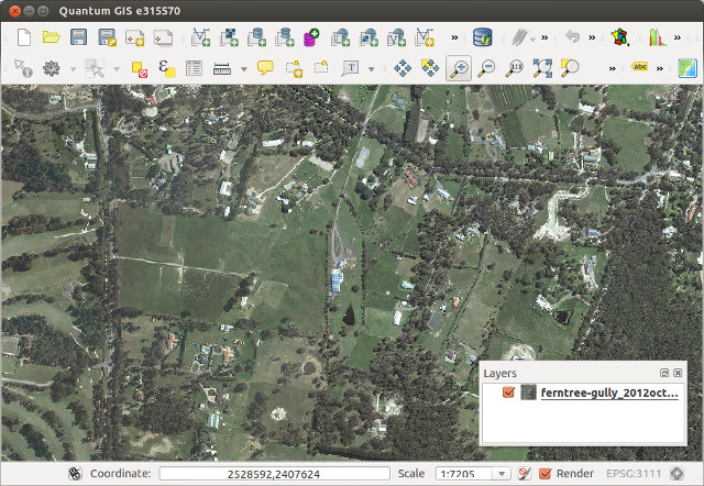
Raster layer before saturation controls…

Let’s tweak the saturation a bit to see if we can make it more appealing. In the Style tab under raster layer properties, you’ll see a new “Saturation and hue” section. For this layer I’ll bump the saturation up from its default value of zero:
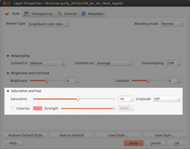
Saturation settings

Saturation settings

Which results in something like this:

Resultant layer!

… and after increasing the saturation!

Ah, much better. This actually looks like somewhere I’d like to live. A bit over-the-top perhaps, but it IS handy to make quick adjustments to raster colours in this way without the need for any external programs.

How about turning an image grayscale? I regularly have to do this with street directory basemaps, and until now couldn’t find a satisfactory way of doing this in QGIS. Previously I’ve tried using various command line utilities, but never found one which could turn an image grayscale without losing embedded georeferencing tags. (I did manage to achieve it once in QGIS using a convoluted approach involving the raster calculator and some other steps I’ve thankfully forgotten.)

But now, you can forget about all that frustration and quickly turn a raster grayscale by using a control right inside the layer properties! You even get a choice of desaturation methods, including lightness, luminosity or average. Best part about this is you can then right click on the layer to save the altered version out to a full-resolution georeferenced image.

grayscale

Street map in grayscale… woohoo!

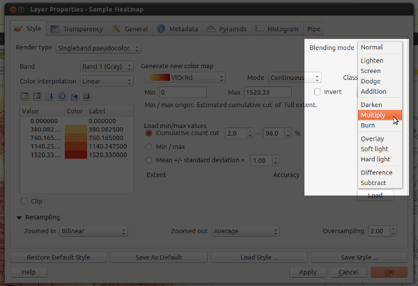
Lastly, there’s the colourise option. As expected, this behaves in a similar fashion to the colourise tools in GIMP and Photoshop. It allows you to tint a layer to a specified colour. Let’s take a WMS layer of Melbourne, tweak the brightness and contrast, and colourise it blue…

colorize_settings

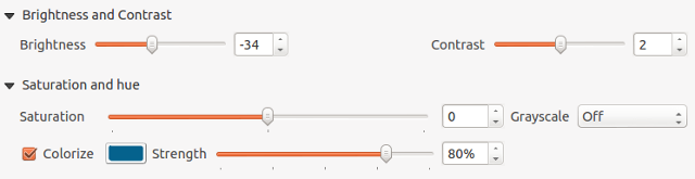
Tweaking the colourize settings

… and the end result wouldn’t be out of place in Ingress or some mid 90’s conspiracy flick!

colorized

Colorized WMS layer

These changes are just a tiny, tiny part of what QGIS 2.0 has to offer. It’s looking to be a sensational release and I can’t wait for final version in June!

Tagged , , , , , , , ,

Coming soon in QGIS 2.0 – blend modes for layers

I’ve just pushed my first major contribution to QGIS — the ability to set the compositing mode for a layer. Compositing is a technique widely used by cartographers and graphic artists to fine tune how layers are blended together, and it allows for some spectacular results! Until now, the only way to get these effects would be to export a map to a separate editor like Photoshop or GIMP and playing with the layer modes there. But with QGIS 2.0, blending can be controlled via a simple drop down menu for both raster and vector layers:

Blending modes for a raster layer

Woohoo… blending modes in QGIS!

So what makes this so great? Well, in previous versions the only option for compositing layers in QGIS was by setting a layer’s opacity. This approach has some limitations. Let’s say you want to overlay two raster layers – a basemap layer and a heatmap. You could place the heatmap layer over the basemap and set its transparency at 50% so that the basemap shows through, but then both the basemap and heatmap layers will be partially faded out:

Overlaying layers with transparency

Overlaying layers by altering transparency – see how both the heatmap and basemap are partially faded

With QGIS 2.0, you’ll be able to use the “multiply” blend mode to overlay these layers. This means both the heatmap and underlying basemap will be shown with full intensity:

Overlaying rasters with multiply

Overlaying rasters with “multiply” blend mode – both layers are shown in their full intensity!

Ok… perhaps that’s not the prettiest example, but it is something I have to do a lot in my job. Until now it’s only been possible by exporting the map to GIMP or Photoshop/Illustrator and setting the blend modes there. That’s always fiddly, time consuming and generally frustrating all round. Much easier to just change it with a dropdown within QGIS itself.

Let’s move on to some more impressive example. First, here’s a terrain map using a combination of a landcover thematic with ‘overlay’ blending and a hillshade set to ‘multiply‘ blending. The graticule lines are also set to overlay – note how they aren’t visible over the lighter water areas and brighter hillshade regions.

Hill shading with advanced compositing

Hill shading with advanced compositing… Hal Shelton would be proud!

Ok, that’s nice, but let’s try something a little different. Using a combination of darkenscreenhard light and overlay:

Stamen-style watercolors directly within QGIS!

Live Stamen-style watercolors within QGIS – sweet!

These a just some rough examples — I’m keen to see what results others get using this feature (feel free to post links to your work in the comments).

One final note: I’m really appreciative of the efforts of the QGIS dev team, who’ve been really supportive and helpful while I find my way around the QGIS codebase. A big thank you has to go to Nathan Woodrow for taking the time to review this commit and answering all the questions I’ve had!

Tagged , , , , ,

Random Hack: Fixing triplej’s Movie Guy podcast

I’m a huge fan of Marc Fennell’s movie reviews on triplej. The guy really seems to nail it — it’s not often I disagree with his opinion on a film. Triplej have even made it easy for me to catch up with his reviews, even though I hardly ever get a chance to listen to the radio anymore.

Actually, I need to correct that – they’ve made it only somewhat easy. For some bizarre reason someone has made the obscure decision that all the dates in his podcast should be one year in the future:

The magical time travelling podcast

That’s right, it’s a magical time travelling podcast

This has the annoying effect of totally breaking episode sorting in every podcast app. Episodes from this feed will always appear above episodes from any other subscriptions, even if the episodes are actually a year old.

When I first noticed this I assumed it was only a temporary error which would be fixed quickly. That was over two years ago. So, this week I finally decided to do something about it. I’ve whipped up a small php script which fetches the feed from the triplej website and subtracts one year from every date on the podcast. The resultant fixed feed is now available here, all ready to be safely subscribed to without breaking the temporal rules of the universe.

I’m not sure if any other podcasts on the triplej site suffer from this same issue. If you’ve come across any others leave me a comment and I’ll implement the same fix for it!


Tagged , ,

Fuzzy string matching and geocoding

One of the biggest problems encountered when trying to geocode a table is how to handle variations in spelling and naming between points. Databases are often messy, filled with spelling and typing mistakes – and this makes it impossible to simply match one table against another. That’s when we need to resort to the concept of “fuzzy string matching” – the “technique of finding strings that match a pattern approximately (rather than exactly)” 1.

The traditional method for fuzzy string matching during geocoding is the Levenshtein distance. The Levenshtein distance is perfect for automatically correcting spelling mistakes and small variations in spelling (eg  “Frankston-Flinders Rd” as opposed to “Frankston Flinders Rd“). When geocoding, you can automatically match any results with a distance of just 1 or 2 characters, or which is within a set percentage of the length of a string. For instance, the Levenshtein distance between “Swanton St” and “Swanston St” is one character (10% of the length of the first string), and the distance between “Box Hil Railway-Station”  and “Box Hill Railway Station” is two characters (~8.5% of the length of the first string). I’ve found that automatically matching distances between 1 character and 10% of the string length covers most simple typing errors with almost no false matches.

Unfortunately, the Levenshtein distance isn’t perfect. While it works well when the strings only contain small differences, it fails when trying to match two very different strings. This becomes critical when we’re trying to match the names of features. There’s often a huge variety in possible names for features. A train station could be entered as any number of different names, ranging from  “Box Hill Railway Station“, “Box Hill Train Station“, “Box Hill Station“, all the way to “Railway Station, Box Hill” or just “Railway Station“.

Let’s try a possible example. Trying to match the string “coles” to the name “coles supermarket” will have the high Levenshtein distance of 12 characters. By comparison, the Levenshtein distance between “coles” and “fat apes” is only six characters. If we are ranking matches by Levenshtein distance alone we’ll end up choosing the match “fat apes” over the obviously more relevant match of “coles supermarket“. Not terribly effective at all…

A better technique to use for matching these feature names is the the algorithm called “longest common substring2. This algorithm returns the longest string which is common to both input strings. Taking our previous examples, when matching “coles” to “coles supermarket” the longest common substring (LCS) is “coles“. Comparing “box hill railway station” to “railway station, box hill“, the LCS is “railway station“.

I’ve found that using the longest common substring for geocoding works best interactively. First, you take the string you’re trying to match, and sort a list of possible candidates by the length of the LCS, with longest matches first. This sorted list is then presented to the user to manually choose the most appropriate match.

Why not just do this automatically, without bothering the user? While most times the best match will be the first one in the list, there’s a few times when it may be second or third. Let’s say we’re trying to match the string “coles supermarket, westfields shopping centre”, and our feature database contains a specific point for “coles supermarket” and a general point for “westfields shopping centre”. If we were to automatically match to the point with the largest LCS, we’ll end up matching to the general point “westfields shopping centre” (LCS length of 26), rather then the slightly more accurate point for “coles supermarket” (LCS length of 17). Unfortunately, I can’t think of an automated way of prioritising the specific point over the general point in this case, so it’s safest to leave that choice to the user. (Let me know if you’ve got any clever ideas for this!)

This method can be taken one step further by padding both strings with a space. This has the effect of increasing the length of the LCS if both input strings match on a full word. For example, the LCS between “coles supermarket” and “coles” has length 5, while the longest common substring between “coles supermarket” and “dandenong markets” has length 6. If we just choose to use the standard LCS method on these strings we’ll incorrectly prioritise “dandenong markets” over “coles“. However, if we append spaces to the start and end of the strings, then we get:

" coles supermarket " and " coles ", LCS = " coles ", length 7
" coles supermarket " and " dandenong markets ", LCS = "market", length 6

Effectively, this process bumps up the length of an LCS by two characters if both input strings match with word breaks, rather than a portion of a word. It’s also possible to replace every space in the input strings by multiple spaces, if you’d like to further prioritise whole word matches.

In summary – Levenshtein distance is great for small variations in names, but for large possible variations in naming I’ve found LCS to be much more effective.

Notes:

  1. http://en.wikipedia.org/wiki/Approximate_string_matching
  2. Watch out, there’s a similarly named algorithm called “longest common sub sequence”. You don’t want this one at all.
Tagged , , , ,

RMIT Crime Mapping and Analysis Conference 2012

This is just a quick plug for the first RMIT Crime Mapping and Analysis Conference, which is happening in Melbourne next week (13-14 November). There’s some great international speakers like Spencer Chainey presenting. I’ll also be giving a short talk on predictive mapping in policing, using a residential burglary forecasting model as a case study. More details and pricing is available on the conference site.

Tagged

Leaflet and Vicgrid (EPSG:3111) projection

While Leaflet is a fantastic mapping library, there’s not a lot of info out there on how to use it with different projections. I thought I’d share some tips I discovered while trying to get Leaflet working with a WMS server that only supports the projected VICGRID94 (EPSG:3111) CRS. Leaflet’s documentation is generally OK, but there’s a few potential roadblocks which took me a while to understand.

First you’ll need Leaflet, proj4js and Proj4Leaflet all installed on your server and linked to your page.

Before you initialise the map instance you’ll need to set up the CRS transform, which goes along the lines of:

// Coordinate to grid transformation matrix
var transformation = new L.Transformation(1, 0, -1, 0);
// Official Spatial Reference from http://www.spatialreference.org/ref/epsg/3111/
var crs = L.CRS.proj4js('EPSG:3111',
'+proj=lcc +lat_1=-36 +lat_2=-38 +lat_0=-37 +lon_0=145 +x_0=2500000 +y_0=2500000 +ellps=GRS80 +towgs84=0,0,0,0,0,0,0 +units=m +no_defs',
transformation);

You’ll also need to set up scale function, and assign it to your crs object.

// Scale for each level
var res = [2116.670900008467, 1058.3354500042335, 529.1677250021168, 264.5838625010584, 132.2919312505292, 66.1459656252646, 26.458386250105836, 13.229193125052918, 6.614596562526459, 2.6458386250105836, 1.3229193125052918, 0.6614596562526459, 0.33072982812632296, 0.21166709000084669];

var scale = function(zoom) {
 return 1 / res[zoom];
}
crs.scale = scale;

It took me a while to track this one down, but when you’re creating your layers, make sure you set “continuousWord: true” . Failing to set this will result in no tiles being loaded. Here’s an example WMS layer:


var cartolayer = L.tileLayer.wms("http://x.x.x.x/map/wms", {
 layers: 'basemap',
 format: 'image/png',
 continuousWorld: true,
});

Lastly, when initialising the map:

  • You must again set the option continuousWorld: true
  • You must set “worldCopyJump: false”, or you’ll have problems with the map jumping to a random location when you attempt to drag it (see Leaflet issue #1003)
  • Set the crs to the one created earlier
</pre>
var map = new L.Map('map', {
 crs: crs,
 continuousWorld: true,
 center: new L.LatLng(-37.8, 144.9),
 zoom: 5,
 minZoom: 0,
 maxZoom: 13,
 worldCopyJump: false
});

Now you should be right to go and take advantage VICGRID with all that Leaflet goodness!

Some information which might be useful is available at:

Tagged , , , , ,

Investigating MapInfo’s Geocode Routine

After doing a bit of work using MapInfo’s built-in Geocode routine I started getting curious about how the routine handles various special cases. After a bit of experimenting I thought I’d document what I found out.

Starting with the simplest case, a street with odd numbers (1-9) on the left, and even numbers (2-10) on the right. The red stars show where MapInfo geocodes house numbers 3 and 4:


So far so good – we can see that MapInfo has correctly determined that one side of our street corresponds to odd numbers and one to even, and it has correctly matched the address points to the corresponding side of the road. Let’s try a one sided road next:

MapInfo treats -9999 values in an address ranges table as “no address points”. This road segment is correctly handled by MapInfo, and house number 4 gets geocoded to the correct side of the road. Nothing unexpected so far, but now let’s split the street into two lanes, with odd numbers on one side and even on the other:

More or less what we want to see. I should point out that in all these tests I’ve left the default setting of insetting addresses 15% from the ends of the street, which explains why points 2/10 and 1/9 don’t fall right on the beginning and end of the road segments. I’m not sure why the points curve out and fall at varying distances to the road — but it’s close enough and I can live with that.

Just to see what happens, lets go back to one road segment with valid even numbers (2-10) on only one side, and try geocoding an odd number house (9):

MapInfo has geocoded the point right in the centre of the road segment. Not what we’d like, but at least the Find command returns a result of 11 (exact match, side of street undetermined) for this case and it’s possible to find and avoid these types of errors. What happens now if we mix odd and even numbers on the same road side?

Here we’ve set one side of the road to range from 1 to 10, and the other to contain no addresses (-9999). Unfortunately none of the house numbers, either odd or even, match correctly in this case. All numbers from 1-10 are placed at the centroid, with a result code of 11. I guess mixing odd and even numbers in a street segment like this should be avoided.  If you have a street segment which does contain a range of odd and even numbers in reality, it looks like the only way to get this to work correctly is to duplicate the road segment, once with an odd number range and once with an even range. Hmmm… I wonder what happens if we have two matching street segments, one with this mix of odd and even numbers, and the second with just odd numbers?

Good – that’s encouraging to see. MapInfo can match the odd numbered houses to the segment with an odd address range of 1-9, even when we have a bad segment which covers the same number range. The even numbers don’t return a match, with a result code of -411 (multiple matches, side of street undetermined, exact match). Let’s take a step back and try a different type of conflict, where the address numbers on either side of the road overlap:

After a bit more testing (which I won’t go into here), it looks like when there’s an overlapping range like this and an address point could fall on either side of the road, MapInfo places it on the right hand side. For reference, overlapping ranges across two different road segments will geocode points which unambiguously fall on one road segment, and return a code of -401 (multiple matches, exact match) for the others:

(Address points 2 and 10 geocode, whereas 4, 6 and 8 don’t). One last thing to try – let’s see what happens when the address ranges table contains a point object. In this case we’ll add a point object with a left range of 1-9 and a right range of 2-10.

I wasn’t expecting this to work, but it appears to correctly geocode any numbers between 1 and 10 directly to the same location as the address ranges point. This is great news (for reasons I’ll possibly go into in a later blog post).

Quick Summary:

  • Don’t have an address range on the one side of a segment which consists of both odd and even numbers. If you do need to have a segment like this, you’ll need to duplicate the segment with one row having and odd range and the other having an even range.
  • Make sure to correctly handle any matches with a result code of side of street undetermined, since these may have just matched to the centre of the road
  • It’s OK to have point objects in an address ranges table
Tagged , , ,

Alpha Shapes for MapInfo

One recurring question which pops up on the MapInfo mailing list relates to creating a polygon which encloses a set of objects.  While this can sometimes be achieved with a Convex Hull, the results aren’t always that useful. For example, take a bunch of points in the shape of the letter A:

Using the standard Convex Hull creates a polygon which totally encloses all these points. However, the polygon doesn’t closely follow the visual shape of the points and covers a much larger area then one would expect:

Convex hull

Alpha shapes are an alternative solution to polygon wrapping. An alpha shape will wrap the input points in a different manner to convex hulls, which more closely follows the ‘visual’ outline created by the points:

Alpha Shape

Mathematically, the concept of alpha shapes is well defined and they can be easily created from subsets of the Delaunay triangulations of an input set. Unfortunately, MapInfo doesn’t include any built-in methods for creating Delaunay triangulations, but it does have a tool for creating Voronoi diagrams. Lucky for us it’s possible to transform a Voronoi diagram into Delaunay triangles.

Ok, now all that background information is out of the way, it’s time to announce mi-alphashapes, a MapBasic based tool for creating alpha shapes in MapInfo!

mi-alphashapes in action

To use, simply load the mbx file and choose Alpha Shapes from the menu. You’ll need to enter an appropriate alpha value – larger values will cause the resultant polygon to behave more like a Convex Hull, smaller values will wrap the points more tightly but may result in multiple shapes. While the extension automatically calculates a sensible default value, you may need to experiment with this to get the best results. This is easy under MapInfo 10.5+, since the extension includes a handy preview window. Additionally, the tool also includes a routine for creating Delaunay triangulations.

Warning: You may run into problems if you’re not using projected coordinates.

I’ve uploaded all the source to GitHub, under a Public Domain license. Feel free to do with it what you will. Otherwise, compiled versions for both MapInfo 8.5+ and MapInfo 10.5+ are available here.

Tagged , ,

Better Dialogs in MapBasic

Any easy way to add some extra polish to MapBasic applications is to switch from using the MapBasic Note and Ask commands to standard Windows message boxes. While the Note command is handy for quickly giving feedback to a user, there’s zero options for customising the dialogs.

Standard MapBasic “Note” dialog – limited to an exclamation icon and “MapInfo” title bar

Let’s see what we can do about that. We’ll start by including a reference to the standard Windows dialog, which is included in the User32.dll library. I also use two tiny wrapper sub/functions (called MessageBox and MsgBox respectively). The function is used for dialogs which need to return a response (a replacement for the Ask function), and the sub for when the response isn’t important (replacement for Note). Lastly, there’s also a bunch of DEFINEs to make calling the routines more convenient and memorable.

Declare Function MsgBoxA Lib "User32.dll" Alias "MessageBoxA" (ByVal hWnd As Integer, ByVal sTxt As String, ByVal sCaption As String, ByVal iTyp As Integer) As Integer
Declare Function MsgBox(ByVal sTxt As String, ByVal sCaption As String, ByVal iType As Integer) As Integer
Declare Sub MessageBox(ByVal sTxt As String, ByVal sCaption As String, ByVal iType As Integer)
' Messagebox dialog buttons
DEFINE vbOKOnly 0
DEFINE vbOKCancel 1
DEFINE vbAbortRetryIgnore 2
DEFINE vbYesNoCancel 3
DEFINE vbYesNo 4
DEFINE vbRetryCancel 5
' Messagebox dialog icons
DEFINE vbCritical 16
DEFINE vbQuestion 32
DEFINE vbExclamation 48
DEFINE vbInformation 64
' Messagebox default button
DEFINE vbDefaultButton1 0
DEFINE vbDefaultButton2 256
DEFINE vbDefaultButton3 512
DEFINE vbDefaultButton4 768
' MsgBox Returned value
DEFINE vbOK 1
DEFINE vbCancel 2
DEFINE vbAbort 3
DEFINE vbRetry 4
DEFINE vbIgnore 5
DEFINE vbYes 6
DEFINE vbNo 7
'**************************************************************************
' Wrapper for standard Win32 Msgbox function
'**************************************************************************
Function MsgBox(ByVal sTxt As String, ByVal sCaption As String, ByVal iType As Integer) As Integer
 MsgBox = MsgBoxA(WindowInfo(WIN_MAPINFO, WIN_INFO_WND), sTxt, sCaption, iType)
End Function
'**************************************************************************
' Messagebox which doesn't return a value
'**************************************************************************
Sub MessageBox(ByVal sTxt As String, ByVal sCaption As String, ByVal iType As Integer)
 Dim i As Integer
 i = MsgBoxA(WindowInfo(WIN_MAPINFO, WIN_INFO_WND), sTxt, sCaption, iType)
End Sub

Now that we’re all setup, we can duplicate the standard MapInfo message box with the call:

Call MessageBox("Standard Windows message box", "My MapBasic Program", vbExclamation)

Message box with customised title

As seen above, MessageBox is called by passing the text of the dialog, a title caption, and one or more options. In this case we’ve used vbExclamation to copy the appearance of the Note command. Nothing too special yet, but let’s explore a little further. In some cases (such as notifying the user when an operation has successfully completed) the exclamation icon just looks wrong. Compare:

Sometimes the exclamation icon isn’t the best choice…

To the dialog created by the code

Call MessageBox("Processing Complete!", "Friendlier Dialog", vbInformation)

Much friendlier!

Let’s take the other extreme, when you need to let the user know that something really bad happened:

Call MessageBox("Something really bad happened..!", "Error", vbCritical)

Guaranteed to get attention!

The other way to use the Message Box is through the MsgBox function. This can be used to ask the user for a response, in a similar way to MapBasic’s Ask function. The big difference is that MapBasic’s Ask dialog causes your eyes to bleed:

MapBasic’s Ask dialog… what’s with all the empty space?

Let’s replace this with a standard Windows message box:

iResponse = MsgBox("Would you like to continue?", "Messagebox with two buttons", vbYesNo + vbQuestion + vbDefaultButton1)
If iResponse = vbYes Then
  ' User clicked yes
ElseIf iResponse = vbNo Then
  ' User clicked no
End If

The code above demonstrates how dialog attributes can be combined:

vbYesNo + vbQuestion + vbDefaultButton1

and how the value returned by the dialog can be checked against the vbYes and vbNo constants to determine the user’s response. Chaining options together allows for very flexible, user-friendly dialogs.  Again, the result looks much nicer (and more professional) then the built-in MapBasic function:

Using a Message Box to ask a question

So there you go! A simple little change you can make to your MapBasic programs to make them just a bit more user-friendly.

Tagged ,

Bluray Ripping Workflow

My workflow for ripping bluray discs. Works for me, and meets all my needs (HD playback via XBMC, SD copies compatible with both iOS and Android). I’m recording it here because it’s about the third time I’ve had to re-work this out…

  1. Rip to mkv using MakeMKV
    • If only DD5.1 track, select it
    • If both DTS & DD5.1 track, select both
    • Select english subtitles, and option for forced subtitles for each subtitle track
  2. Check resultant MKV
    • Make sure DD track is proper movie audio, not commentary
    • Find out if foreign language subtitle track exists
    • Switch on each subtitle track in turn, if english track or closed caption then ignore
    • Rip subtitle track from MKV using MKVtoolnix with MKVExtractGUI2 (windows) to .SUP file
    • If unsure, use Subtitle Edit (windows) to check subtitle track content.
  3. If foreign language subtitles found
    • Convert from SUP to SUB/IDX using BDSup2Sub
    • Insert IDX back into MKV using MKVtoolnix
    • Add original MKV and .idx file. This step converts the subtitles into a format Handbrake can work with (subtitle now in SSA format)
  4. Convert MKV using Handbrake
    • If no DD audio, convert to MKV with DTS audio
    • If DD audio, convert to MP4. Create additional downmixed stereo track
    • RF 18, no downsize
    • Standard def copy: 576p high, RF 20. Only downmixed audio. MP4 format
  5. Use Subler (OSX) to add metadata to mp4 files